요즘 칼만 필터를 공부할려고 하는데.. 생각보다 어렵다...
논문을 봐도 바로 이해가 안가는건 나뿐인건가...ㅡ,.ㅡ;; 젠장..
자료정리는 나중에 하기로 하고 일단.. 긁어보자.
Kalman Filter
Rudolf E. Kalman 이 발명한 칼만필터는 최소자승법 (Least Square Method) 를 사용해서 실시간으로 잡음 (noisy) 운동 방정식 (equations of motion) 을 가진 시간에 따른 방향 (time-dependent state vector) 를 추적하는 효율적인 재귀 계산법 (recursive computational solution) 이다. 칼만필터는 하나의 시스템이 시간에 따른 변화를 적절하게 예측할 수 있도록 잡음 (noise) 으로부터 신호 (signal) 를 찾아내기위해 사용된다.
실제로는 Peter Swerling 이 일찌기 유사한 알고리즘을 개발했다. Stanley Schmidt 는 최초로 칼만필터를 실제로 응용하여 사용했다고 알려져있다. Kalman 이 NASA Ames Research Center 를 방문했을 때 우주선 아폴로의 궤도를 추정하는 문제에 그의 아이디어가 사용될 수 있다는 것을 알게되었고, 우주선 아폴로의 운행컴퓨터 (navigation computer) 에 포함되게 되었다.
다양한 종류의 칼만필터가 지금까지 개발되었는데, 소위 simple Kalman filter 이라 불리우는 칼만의 원래의 형식에서부터, Schmidt 의 extended filter, information filter, Bierman 과 Thornton 등등에 의해 개발된 다양한 squrar-root filter 들이 있다. 칼만필터는 제어시스템공학에서 광범위하게 사용된다. Wiener filter 와 비교된다. ...... (Wikipedia : Kalman filter)
대부분의 사람들은 칼만 필터에 대해 들어 보지 못했다. 그것은 비행기와 우주 탐사 로켓, 그리고 순항 미사일을 유도하고, 위성과 경제의 추세와 혈액 흐름의 변화 등을 추적한다. 그것은 '최적의' 예측기이다. 그것은 비행기가 구름에 가리어 있을 때 비행기의 방향에 대해 '가장 잘' 예측할 수 있도록 한다. 여러분은 어떻게 미사일이 목표물을 찾고, 어떻게 우주 비행사들이 지구로 돌아오는지 궁금해해 본 적이 없는가? 칼만 필터는 어떻게 이러한 일이 가능한지 보여 준다. 다윈의 적자 생존 이론이 진화 생물학을 대표하는 것과 마찬가지로, 칼만 필터는 대부분의 공학을 대표한다. 수천 명의 엔지니어들은 칼만 필터에 약간 덧붙이거나 변형된 논문들을 발표하였다. ..............
term :
예측 (Prediciton) Rudolf E. Kalman 제어 (Control)
Site :
Paper :
칼만필터를 이용한 우리나라의 잠재적 GNP 추정과 경기변동의 추이에 관한 연구 (Potential GNP and Business Cycles of Korea : A Kalman Filtering Approach) : 이병완, 한국경제학회, 1994
확장 칼만필터를 이용한 LEO 위성의 궤도 결정 방법 (THE ORBIT DETERMINATION OF LEO SATELLITES USING EXTENDED KALMAN FILTER) : 최규홍, 손건호, 김광렬, 한국우주과학회, 1995
칼만필터를 이용한 레이다 추적계의 비교연구 : 위상규, 임청부, 한국항공우주학회, 1989
적응 칼만필터를 이용한 MTI 레이터의 이동표적 추적 기법 (Moving Target Tracking Technique of MTI Radar Using Adaptive Kalman Filter) : 박인환, 조겸래, 조설, 한국항공우주학회
칼만필터를 이용한 최고/최저 기온예보 (The Forecasting the Maximum / Minimum Temperature Using the Kalman Filter) : 이동일, 이우진, 한국기상학회, 1999
칼만필터를 이용한 무궁화위성 궤도 결정 성능분석 연구 (Performance Analysis of Kalman Filter Based KOREASAT Orbit Determination) : 박봉규, 안태성, 한국항공우주학회, 2000
반복적 확장 칼만필터를 이용한 얼굴의 3차원 움직임량 추정 (3-D Facial Motion Estimation Using Iterative Extended Kalman Filter) : 박강령, 김재희, 한국정보처리학회
최소 최대 추정량과 베이즈 추정량으로서의 Kalman 필터에 관하여 (On the Kalman Filter as the Bayes Estimator and the minimax Estimator) : 김지곤, 상명대 자연과학연구소, 1998
출처 : Tong - gayanim님의 image processing통
------------------------------------------------------------------------------------------------
Introduction
To many of us, kalman filtering is something like the holy grail. Indeed, it miraculously solves some problems which are otherwise hard to get a hold on. But beware, kalman filtering is not a silver bullet and won’t solve all of your problems!
This article will explain how Kalman filtering works. We’ll use a more practical approach to avoid the boring theory, which is hard to understand anyway. Since most of you will only use it for MAV/UAV applications, I’ll try to make it look more concrete instead of puzzling generalized approach.
Make sure you know from the previous articles how the data from “accelerometers” and “gyroscopes” are used. Some basic knowledge of algebra may also come in handy :-)
Basic operation
Kalman filtering is an iterative filter that requires two things.
First of all, you will need some kind of input (from one or more sources) that you can turn into a prediction of the desired output using only linear calculations. In other words, we will need a lineair model of our problem.
Secondly, you will need another input. This can be the real world value of the predicted one, or something that is a good approximation of it.
Every iteration, the kalman filter will change the variables in our lineair model a bit, so the output of our linear model will be closer to the second input.
Our simple model
Obviously, our two inputs will consist of the gyroscope and accelerometer data. The model using the gyroscope data looks like this:
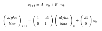
The first formula represents the general form of a linear model. We need to “fill in” the A en B matrix, and choose a state x. The variable u represents the input. In our case this will be the gyroscope’s data. Remember how we integrate? We just add the NORMALIZED measurements up:
alpha k = alpha k-1 + (_u_ k – bias)
We need to include the time between two measurements (_dt_) because we are dealing with the rate (degrees/s):
alpha k = alpha k-1 + (_u_ k – bias) * dt
We rewrite it:
alpha k = alpha k-1 – bias * dt + u k * dt
Which is what we have in our matrix multiplication. Remark that our bias remains constant! In the tutorial on gyroscopes, we saw that the bias drifts. Well, here comes the kalman-magic: the filter will adjust the bias in each iteration by comparing the result with the accelerometer’s output (our second input)! Great!
Wrapping it all up
Now all we need are the bits and bolts that actually do the magic! These are some formulas using matrix algebra and statistics. No need right now to know the details of it. Here they are:
| u = measurement1 | Read the value of the last measurement |
| x = A · x + B · u | Update the state x of our model |
| y = measurement2 | Read the value of the second measurement/real value. Here this will be the angle calculated from our accelerometer. |
| Inn = y – C · x | Calculate the difference between the second value and the value predicted by our model. This is called the innovation |
| s = C · P · C’ + Sz | Calculate the covariance |
| K = A · P · C’ · inv(_s_) | Calculate the kalman gain |
| x = x + K · Inn | Correct the prediction of the state |
| P = A · P · A’ – K · C · P · A’ + Sw | Calculate the covariance of the prediction error |
The C matrix is the one that extracts the ouput from the state matrix. In our case, this is (1 0)’ :
alpha = C · x
Sz is the measurement process noise covariance: Sz = E(zk zkT)
In our example, this is how much jitter we expect on our accelerometer’s data.
Sw is the process noise covariance matrix (a 2×2 matrix here): Sw = E(x · xT)
Thus: Sw = E( [alpha bias]’ · [alpha bias] )
Since only the diagonal elements of the Sw matrix are being used, we’ll only need to know E(alpha2) and E(bias2), which is the 2nd moment. To calculate those values, we’ll need to look at our model: The noise in alpha comes from the gyroscope and is multiplied by dt2. Thus: E(alpha2) = E(u2)· dt2.
These factors depend on the sensors you’re using. You’ll need to figure them out by doing some experiments. In the source code of the autopilot/rotomotion kalman filtering, they use the following constants:
E(alpha2) = 0.001
E(bias2) = 0.003
Sz = 0.3 (radians = 17.2 degrees)
Further reading
'Robotics > Control Tech.' 카테고리의 다른 글
| Robot Motion Planning and Control (0) | 2009.08.22 |
|---|---|
| Robust Trajectory Generation At Singularities (0) | 2009.03.17 |
| 모바일로봇 Localization과 Mapping 강의자료 (0) | 2008.12.10 |
| PID 제어기 개념 및 튜닝 (3) | 2008.12.03 |
| Selectively Damped Least Squares for Inverse Kinematics (0) | 2008.11.11 |